The Compositional Leap - Generative AI in Inverse Design Innovation

Recent advancements in the field of neural partial differential equation (PDE) solvers have revolutionized the design paradigm in engineering, particularly in the inverse design approach. The paper Compositional Generative Inverse Design by Wu et al., published in ICLR 2024, revisits the compositional inverse design using diffusion models. This approach outperforms both state-of-the-art generative models and classical PDE solvers by generating plausible and unique designs. This blog post explores the key contributions of this work, focusing on the strategies used to address the common problem of over-optimization and physically implausible design generation.

Introduction

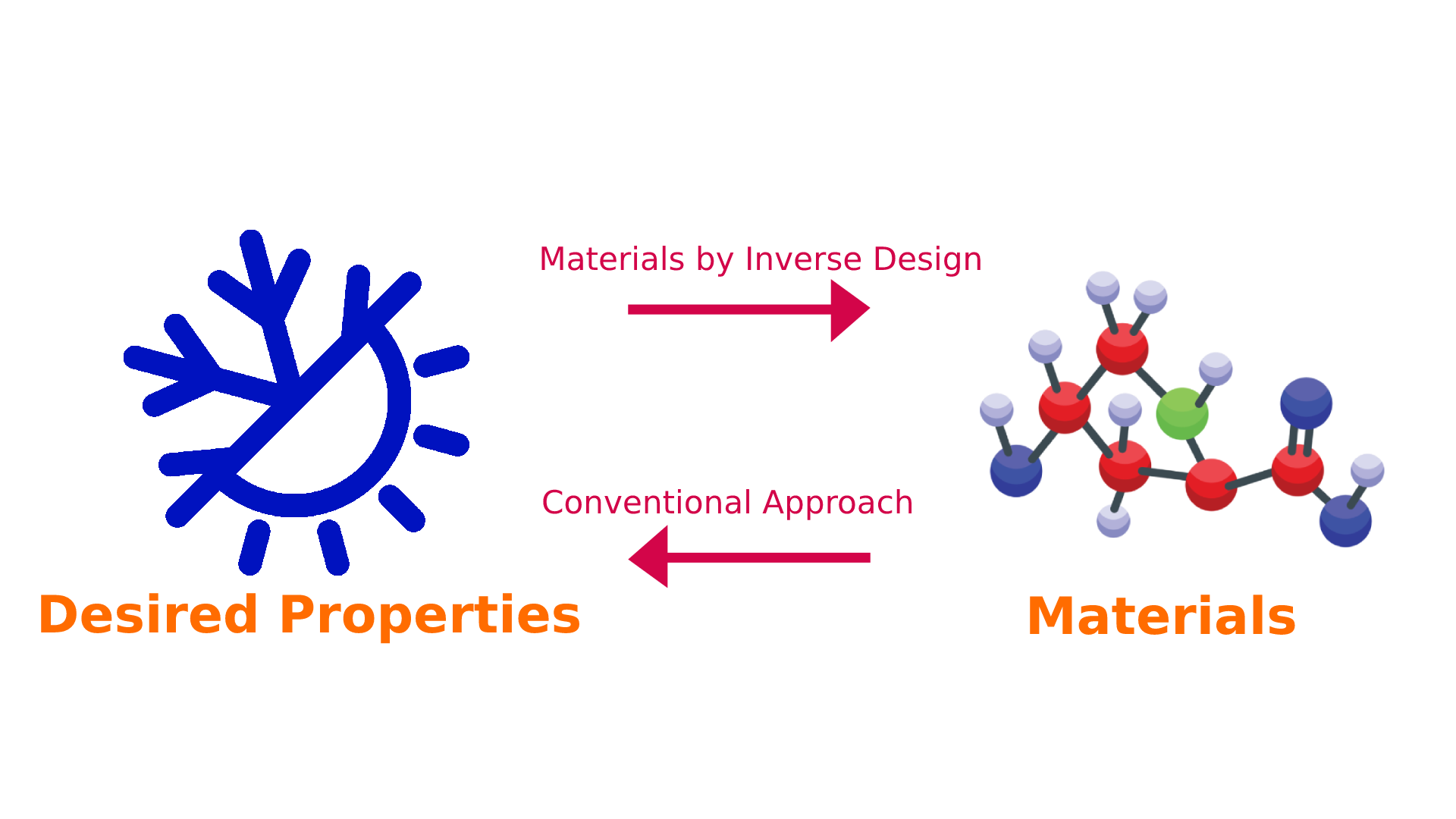
Inverse Design is a paradigm-shifting approach that reimagines traditional optimization. Instead of iteratively refining a system toward a desired outcome, it starts with the end goal itself — a predefined objective — and works backward to computationally derive optimal configurations. This outcome-driven methodology fundamentally reverses the conventional design workflow, prioritizing target specifications over incremental adjustments. For example, in material discovery , instead of starting with a material and calculate its properties, you start with the desired property (like a specific band gap or temperature behavior) and work backward to find or design the material that fits.

The applications of Inverse Design span many domains, including:

Aerodynamics: Designs plane shapes to minimize drag by simulating air-fluid dynamics and boundary interactions.
Underwater Robotics: Optimizes robot shapes for reduced drag, energy efficiency, maneuverability, and acoustic performance.
Nanophotonics: Creates micro- and nano-scale structures for precise light interactions in lasers, data storage, chips, and solar cells.
Battery Design: Enables efficient battery interphases and optimizes charging protocols for high-performance, long-life lithium-ion batteries.

However, inverse design faces challenges related to computational speed due to intensive conventional modeling and optimization, as well as navigating complex, hierarchical, and heterogeneous design spaces. This is especially true for intricate systems, such as rocket designs.

Recent advancements in Generative Artificial Intelligence have opened up new possibilities for solving these problems more efficiently and accurately. AI models can explore high-dimensional spaces, providing unique solutions. However, backpropagation-based inverse design methods, such as the one introduced by Allen et al. , rely on surrogate models that often suffer from adversarial design modes, where the inferred design parameters are not physically plausible despite excellent optimization performance. The method proposed by Wu et al. addresses this issue using compositional diffusion models, which optimize over a learned energy function, improving design stability and generalization.

The background section briefly explains the inverse design problem, followed by a discussion of the Compositional Generative Inverse Design by Wu et al.

Background

The need of Partial Differential Equations (PDEs)

In design optimization, PDEs serve as constraints that ensure the designed system adheres to the governing physical laws. By incorporating PDE constraints, we can accurately predict system behavior under different conditions, leading to designs that are both efficient and feasible. This approach is prevalent in fields like aerodynamics, where optimizing shapes for minimal drag requires solving PDEs that describe fluid flow.

The Basics of PDEs

A Partial Differential Equation (PDE) is a mathematical equation involving an unknown function with several variables and their partial derivatives with respect to independent variables .

Formally, a PDE can be written as:

\[F \left(x_1, x_2, ..., x_n, u, \frac{\partial u}{\partial x_1}, \frac{\partial u}{\partial x_2}, ..., \frac{\partial^2 u}{\partial x_1^2}, \frac{\partial^2 u}{\partial x_1 \partial x_2}, ... \right) = 0,\]

where $u = u(x_1, x_2, ..., x_n)$ is the unknown function, and $F$ is a given function.

Classical Numerical Methods for Solving PDEs

Traditional numerical techniques, such as the Finite Element Method (FEM) and the Finite Difference Method (FDM), have been the cornerstone of PDE solvers . These methods approximate the solution of a PDE by discretizing the spatial domain, converting the continuous problem into a solvable system of equations.

Finite Difference Method (FDM): A grid-based technique that discretizes the spatial domain into a structured mesh and approximates derivatives using finite difference approximations (e.g., forward, backward, or central differences). It is particularly useful for problems where structured grids align well with the computational domain.
Finite Element Method (FEM): Unlike FDM, FEM divides the domain into smaller, simpler elements (such as triangles or quadrilaterals) and represents the solution using basis functions. This method is especially useful for complex geometries where structured grids may not be efficient.

Numerical solvers discretize the continuous spatial and temporal domains into a finite set of points to approximate solutions. Two widely used approaches for domain discretization are:

Eulerian Scheme: A fixed-grid approach that is commonly used in finite difference methods for solving PDEs. The spatial domain is discretized into a structured grid, and differential operators are replaced by numerical approximations. For example, a forward difference approximation for a spatial derivative is:
\[\frac{\partial u}{\partial x} (x, t) \approx \frac{u(x + \Delta x, t) - u(x,t)}{\Delta x},\]
where $\Delta x$ represents spatial grid spacing and $x + \Delta x$ are points on the computational mesh. This approach is efficient for structured problems but struggles with deformable geometries.
Lagrangian Scheme: A finite element-based approach that tracks individual points (particles) as they move through the domain. This method is particularly useful for problems where the computational domain deforms over time, such as fluid dynamics and material simulations. A well-known example is Smoothed Particle Hydrodynamics (SPH) , which approximates fluid behavior using a set of discrete particles. However, SPH and other Lagrangian methods can suffer from challenges like particle clumping and numerical instability.

Limitations of Classical Numerical Methods

Despite their effectiveness, classical numerical methods suffer from several limitations:

High accuracy but low efficiency: While these methods provide precise solutions, they are computationally expensive, making them impractical for real-time or large-scale applications.
Need for rich expert knowledge: Implementing and tuning numerical solvers require deep expertise in numerical analysis, discretization techniques, and domain-specific PDE formulations, making them less accessible.
Difficulty in handling high-dimensional design spaces: Many real-world problems involve complex, high-dimensional parameter spaces, where traditional numerical methods struggle due to the curse of dimensionality and the need for fine discretization.

Time-Stepping Methods

To solve dynamic PDEs, numerical solvers combine time-stepping methods with the previously discussed spatial discretization approaches . These methods advance solutions in time while ensuring stability and accuracy.

Explicit Methods: Directly compute the future state using known values. A common example is the forward Euler method:
\[u_{t+\Delta t} \approx u_t + \Delta t \partial_t u.\]
While simple and computationally efficient, explicit methods require small time steps to maintain stability, especially for stiff PDEs.
Implicit Methods: Solve equations involving both the current and future states, allowing for larger, stable time steps. However, they require iterative solvers, increasing computational cost. Implicit methods are preferred for problems with strict stability constraints, such as fluid dynamics and structural mechanics.

Due to the computational challenges, expert knowledge requirements, and scalability issues of classical numerical methods, researchers have explored alternative approaches. Recent advancements in deep learning-based generative models offer promising solutions, enabling efficient and scalable PDE solvers without the traditional constraints.

Neural PDE Solvers

Deep Learning-based PDE solvers significantly outperform classical numerical methods in terms of speed, scalability, and adaptability. Neural solvers can generalize across conditions, adapt to tasks, and learn directly from data, making them particularly valuable for complex or uncertain systems. They allow for larger time steps, most are meshless, and leverage GPUs efficiently.

Problem Setup

Time-evolving PDEs describe how a system changes over space and time:

\[\partial_t u + \mathcal D (x, t, u, \partial_x u, \partial_{xx}u,...) = 0 \quad (x, t) \in U,\] \[u(x, 0) = u_0(x) \quad x \in \mathbb{X},\] \[\mathcal{B}u(x, t) = 0 \quad (x, t) \in \partial \mathbb{X} \times \mathbb{T},\]

where:

$u(x, t)$ is the unknown function (solution) over space ($\mathbb{X}$) and time ($\mathbb{T}$),
$D$ is the differential operator relating derivatives of $u$,
$u_0$ is the initial condition at $t = 0$,
$B$ represents the boundary condition on the spatial domain’s boundary ($\partial \mathbb{X}$).

The goal is to find $u(x, t;\gamma)$ that satisfies these equations, where $\gamma$ defines the problem setup (initial, boundary condition, and parameters). The objective function $\mathcal{J}$ measures the quality of the design:

\[\dot\gamma = \underset{\dot\gamma}{\arg\min}\, \mathbb{E}_{x,t}[\mathcal{J}(u(x, t; \hat\gamma))]\]

Deep Learning-Based Inverse Design

Recent advancements in machine learning have introduced innovative methods for solving inverse design problems in fluid-structure interactions and other physical systems. A notable approach is presented in the paper Physical Design Using Differentiable Learned Simulators by Allen et al. (2022) . This method leverages graph neural network (GNN) simulators combined with gradient-based optimization to predict the physical dynamics and optimize design parameters.

Method Overview

The figure below outlines the method’s pipeline:

Fig 2 Inverse designing with neural surrogate model

Surrogate Forward Model:
A learned forward model, denoted as $f_\theta$, is trained to autoregressively predict the system’s dynamics over time. Given the initial state $u^0$ and the design parameters $\gamma$, the model predicts the subsequent states $u^1, u^2, ..., u^T$. This forward pass mimics the physical process being simulated.
Optimization via Backpropagation:
Using the predicted dynamics $U_{[0,T]}(\gamma)$, the method evaluates an objective function $J(U_{[0,T]}(\gamma), \gamma)$. The objective is optimized with respect to the design parameters $\gamma$ using backpropagation through time (BPTT). This enables efficient gradient-based updates, allowing the model to adjust $\gamma$ to achieve the desired target dynamics or design outcomes.

Challenges

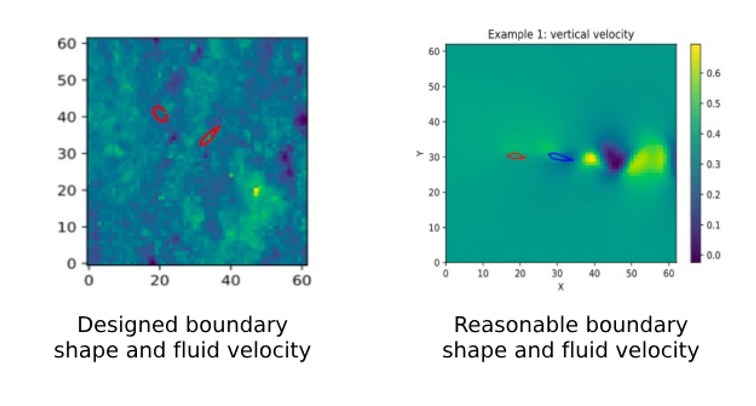
A significant challenge with these models is the risk of over-optimization. This occurs when the optimization process exploits inaccuracies in the surrogate model, leading to design parameters that appear optimal within the model but perform poorly in reality—a phenomenon known as adversarial design parameters . The root cause of this issue is that surrogate models typically lack a measure of data likelihood and cannot discern whether design parameters are within the distribution of the training data. Consequently, optimization can easily venture into regions outside the training distribution, resulting in designs that the surrogate model cannot accurately predict. This limitation underscores the need for methods that can account for data likelihood and maintain optimization within the bounds of the training distribution to ensure reliable performance.

Compositional Models

Compositional models are frameworks that solve complex tasks by decomposing them into smaller, interpretable subtasks, each handled by specialized sub-models. These sub-models are designed to represent distinct concepts, skills, or physical principles, and their outputs are combined—either sequentially or hierarchically—to produce a unified solution. This approach mirrors how humans solve problems by breaking them into modular steps (e.g., “build a chair” → design legs, seat, backrest → assemble parts).

Example: Composable Diffusion Models

A seminal example is Compositional Visual Generation with Composable Diffusion Models by Liu et al. . Here, individual diffusion models are trained to represent specific visual concepts (e.g., objects, textures, spatial relationships).

Applications Beyond Vision

In 3D synthesis, separate models handle geometry, material properties, and physics constraints.

For trajectory planning, sub-models manage obstacle avoidance, dynamic constraints, and energy efficiency.

In hierarchical decision-making, compositionality enables high-level task decomposition (e.g., “grasp object” → plan arm motion, adjust gripper force).

Compositional Inverse Design using Diffusion Models (CinDM)

Wu et al. reimagine inverse design through the lens of diffusion processes, merging the flexibility of compositional energy optimization with the generative power of probabilistic models. Their framework, CinDM, reframes design generation as a guided stochastic exploration of high-dimensional solution spaces, where constraints and objectives act as dynamic sculptors of the diffusion trajectory.

Main contribution:

Novel Inverse Design Formulation: Inverse design is treated as an energy optimization problem, enabling flexible and efficient design generation.
CinDM: Compositional Inverse Design with Diffusion Models, which generalizes to complex and out-of-distribution inputs beyond the training set.

Problem Formulation

This method uses an energy optimization perspective instead of relying on a surrogate model. By formulating this way, the method address a key issue with existing inverse design approaches, where the optimization process can easily fall out-of-distribution of the distribution of the design parameters seen during training.

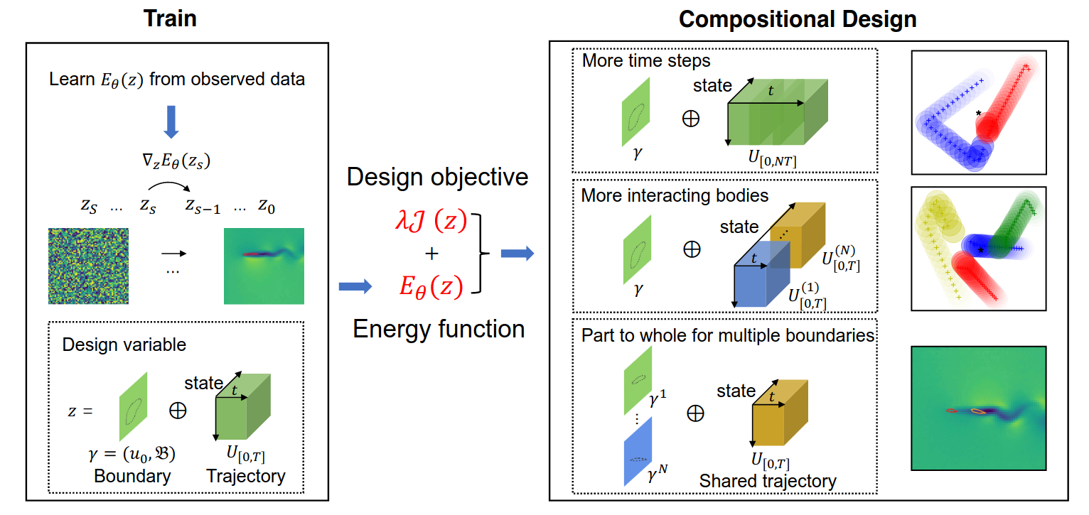
This approach jointly optimize the design objective $\mathcal J$ and a generative objective $E_\theta$,

\[\dot\gamma = \underset{\dot\gamma,U_{[0,T]}}{\arg\min}\, [E_\theta (U_{[0,T]}, \gamma] + \lambda \mathcal J (U_{[0,T]}, \gamma) ],\]

where $E_\theta$ is an energy-based model (EBM) , trained over joined distribution of trajectories $U_{[0,T]}$ (discrete version of $u$ as we don’t have access to ground-truth model for dynamical system) and boundaries $\gamma$ and $\lambda$ is hyperparameter balancing the two objectives.

We also need training loss to that used to train energy-based model $E_\theta$ using a diffusion objective.

\[L_{\text{MSE}} = \| \epsilon - \epsilon_{\theta}(\sqrt{1-\beta_s} z + \sqrt{\beta_s} \epsilon, s) \|_2^2, \quad \epsilon \sim \mathcal{N}(0, I),\]

where:

$\epsilon_{\theta}$ is the denoising network
$z$ represents all variables in the design optimization ($z = U_{[0, T]} ⊕ \gamma$)
$s$ is the diffusion step
$\beta_s$ is a noise schedule parameter
$\epsilon$ is Gaussian noise

The following equation represents a step in the Langevin sampling process used in the optimization . It iteratively updates the optimization variable $z$ to minimize the combined objective.

\[z_{s-1} = z_s - \eta (\nabla_z (E_\theta(z_s) + \lambda J(z_s))) + \xi, \quad \xi \sim \mathcal{N}(0, \sigma_s^2 I),\]

Where:

$z_s$: Current optimization variable.
$\eta$: Step size.
$E_\theta$: Energy function modeling the system.
$J(z_s)$: Design objective.
$\lambda$: Hyperparameter weighting J(zs)J(z_s)J(zs).
$\xi$: Gaussian noise added to explore the space.

Compositional Generative Inverse Design

The method enables generalization to more complex scenarios by composing energy functions $E_\theta$ defined over subsets of the design variables $z$. Each subset enforces local physical consistency while their overlap ensures global consistency.

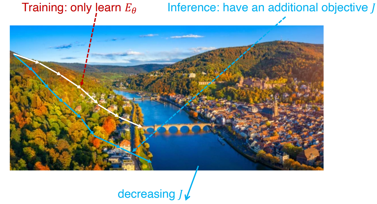
Only energy function $E_\theta$ will be optimized during training. However, during inference time, both objective $J(z_s)$ and energy function $E_\theta$ will be optimized together.

Fig 5 An intuition about getting an unique solution by considering Design Objectives during inference

The pseudo algorithm is given as:

# Compositional Inverse Design with Diffusion Models (CinDM)
# Input: Diffusion models {ϵ_iθ}, design objective J(·), hyperparameters λ, S, K
# Output: Optimized design variables γ and trajectory U[0,T]

initialize z_S ∼ N(0, I)  # Random initialization

# Optimize across diffusion steps S
for s = S, ..., 1:
    # Langevin sampling steps at step s
    for k = 1, ..., K:
        ξ ∼ N(0, σ_s^2 I)  # Sample Gaussian noise
        z_s ← z_s - η * (1/N) * Σ_i [ϵ_iθ(z_s^i, s) + λ ∇z J(z_s)] + ξ
    
    ξ ∼ N(0, σ_s^2 I)  # Noise for next diffusion step
    z_s-1 ← z_s - η * (1/N) * Σ_i [ϵ_iθ(z_s^i, s) + λ ∇z J(z_s)] + ξ

return γ, U[0,T] = z_0  # Return optimized results

Experiments

The study rigorously evaluates CinDM’s ability to generalize across three distinct axes: (1) system complexity, synthesizing configurations with components exceeding training data scales; (2) unseen constraints, adapting to novel physical or geometric requirements not encoded during training; and (3) cross-domain adaptability, transferring learned priors to disparate design problems. These experiments collectively demonstrate how compositional energy guidance in diffusion models enables scalable robustness, outperforming monolithic architectures in handling out-of-distribution challenges.

1. Generalization to Longer Time Steps:

Trajectories are split into overlapping intervals during training.
At test time, the model combines these intervals to generate longer rollouts (e.g., 34, 44, or 54 steps).
This enables accurate design for systems evolving over extended time horizons.

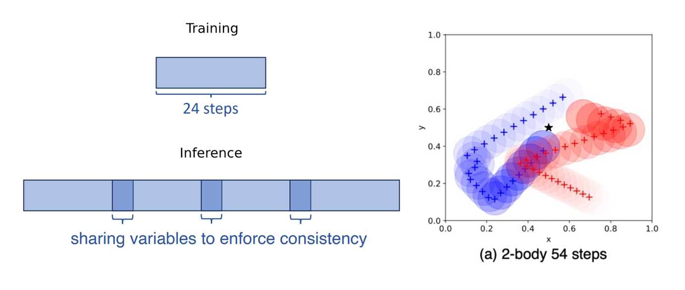
Fig 6 Different time steps during training and inference

CinDM significantly outperformed baselines (CEM , Backprop ) in both trajectory accuracy (MAE) and design objectives.

2. Generalization to More Interacting Objects:

Pairwise energy functions learned from smaller systems (e.g., 2-body interactions) are composed to model larger systems (e.g., 4-body or 8-body).
This allows CinDM to scale and handle more complex dynamics with many interacting entities.

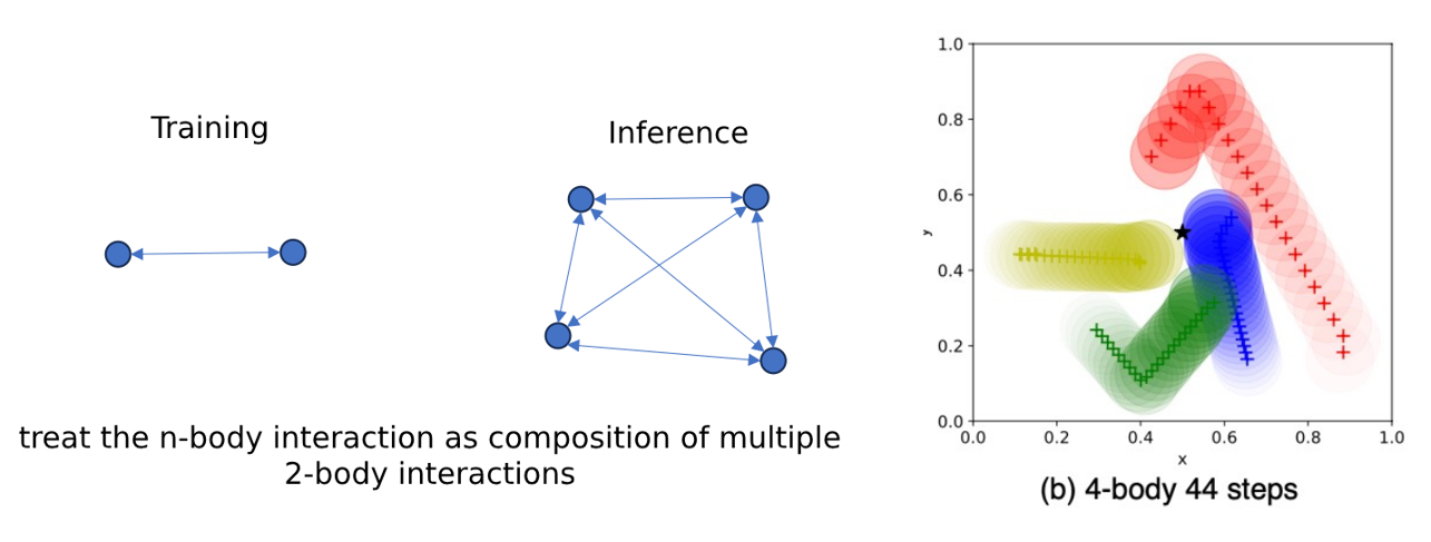
Fig 7 gives Different state composition duringtraining and inference

CinDM excelled at scaling to systems with more interacting bodies (4-body and 8-body), outperforming baselines in both accuracy and design objectives.

Method	4-body, 24 steps (MAE ↓)	4-body, 44 steps (MAE ↓)	8-body, 24 steps (MAE ↓)	8-body, 44 steps (MAE ↓)
Backprop, GNS (1-step)	0.06008	0.30416	0.46541	0.72814
CinDM (Ours)	0.03928	0.03163	0.09241	0.09249

3. Generalization from Parts to Whole for Boundaries:

Design variables (e.g., shapes) are decomposed into parts during training, with individual energy functions for each part.
At test time, the parts are composed into a whole system (e.g., multi-part structures like planes or airfoils).
This supports designing more complex systems by leveraging local consistency across parts.

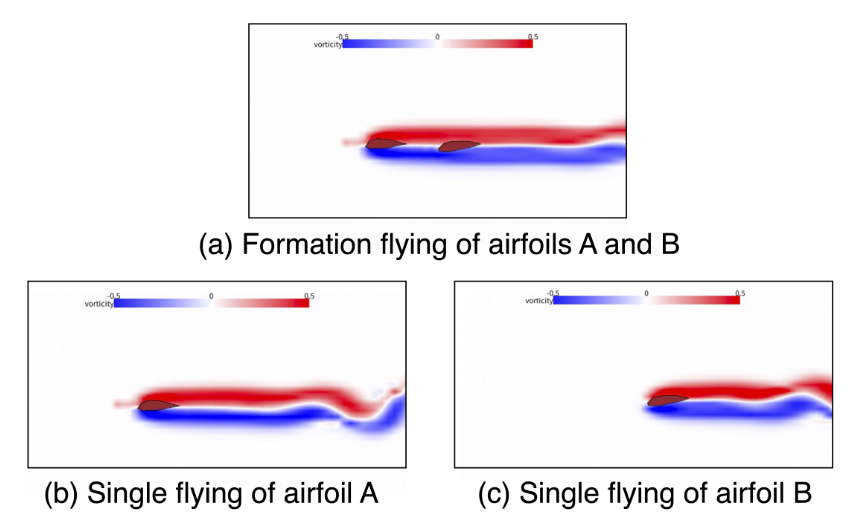
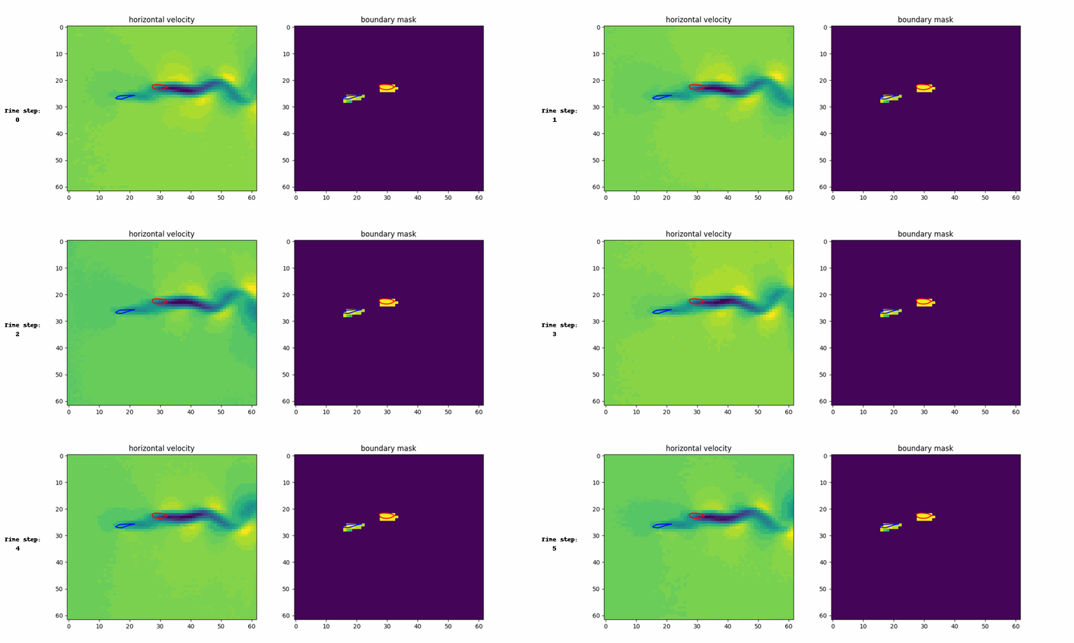
fig 8 Different boundary conditions during inference

CinDM showed superior performance in terms of lift-to-drag ratio and design objective compared to other methods. It also discovered formation flying, reducing drag and increasing efficiency.

Method	1 Airfoil (Lift-to-Drag Ratio ↑)	2 Airfoils (Lift-to-Drag Ratio ↑)
CEM, FNO	1.4005	1.0914
Backprop, FNO	1.3300	0.9722
CinDM (Ours)	2.1770	1.4216

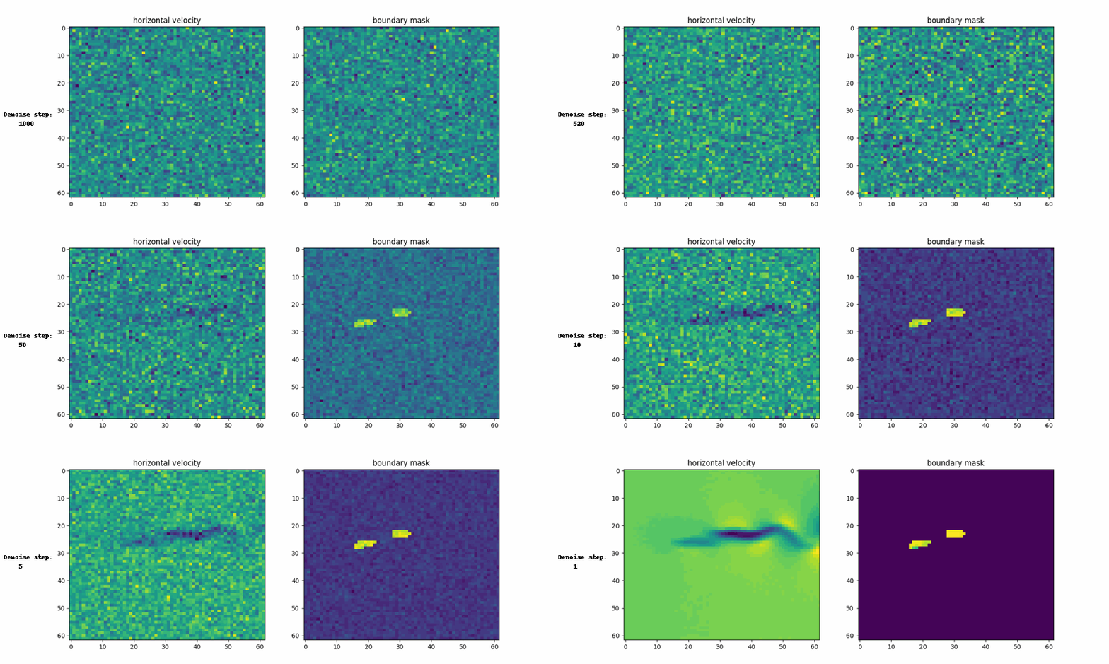
Here are the visual representation of generation process and generated example

Conclusion

The authors conclude that the Compositional Inverse Design with Diffusion Models (CinDM) method offers a novel and effective approach to compositional generative inverse design. This conclusion stems from CinDM’s ability to compose trained diffusion models, focusing on subsets of design variables, and jointly optimize trajectories and boundaries. This allows CinDM to generalize and design systems of greater complexity than those encountered during training.

Key takeaways

Compositionality is key: CinDM’s ability to compose diffusion models trained on simpler design components enables it to tackle more complex systems at test time. This is highlighted by its successful generalization to longer time horizons, systems with more interacting objects, and the design of complex 2D airfoil shapes.
Generative approach for robust design: By framing inverse design as an energy optimization problem within a generative framework, CinDM encourages physically consistent designs and avoids falling into adversarial modes, as observed in some baseline methods.
Wide applicability: The authors believe that the CinDM approach can be applied to a wide range of inverse design problems beyond the examples presented in the sources. They suggest its potential use in material design, drug discovery, and molecule design.

Ongoing Challenges

Complex Design Space: Real-world design problems often involve complex systems with many components that can be combined in various ways. For example, in rocket design, the system includes an airframe, propulsion, and payload, each consisting of hundreds of parts. Representing and optimizing such a complex design space is a significant challenge.
Conflicting Objectives: Engineering designs usually involve multiple objectives that can conflict with each other. For instance, in designing a phone battery, we want it to be both long-lasting and lightweight, but these goals often oppose each other, requiring a balanced solution.
Changing Importance of Objectives: The importance of different objectives can change depending on the situation. For example, during a rocket launch, air resistance, fuel efficiency, and structural durability have different levels of importance as the rocket moves from the ground to space, creating varying optimization priorities.

Remarks

In their paper “Compositional Generative Inverse Design,” Wu et al. introduce a novel approach to inverse design through the use of compositional generative models, leveraging diffusion-based energy functions for optimization. The key contributions of this work are the introduction of a generative perspective to avoid adversarial design and the ability to generalize to more complex and unseen design scenarios, such as longer time steps and systems with more interacting components. The method enables efficient optimization without relying on autoregressive rollouts, and its compositional nature allows for the design of complex systems, like multi-airfoil configurations, by combining simpler learned models. Additionally, the approach introduces a compositional framework that can be applied to a wide range of design tasks, significantly enhancing the flexibility and performance of inverse design solutions.